

In my previous post, I had ended it with a bunch of questions like coming up with a number that could represent the whole data, summarize the information, and on ways to measure them, if they even exist. But do they?
OfCourse these measures exist. Infact these measures have been developed over the course of time since the birth of human civilization and the concept of trade. They are called the averages or measures of central tendency.
But why are they called that?
Professor Bowley states that averages are “statistical constants which enable us to comprehend in a single effort the significance of the whole.” What does he mean?
Central tendency simply refers to the number falling right in the middle or center of the data set. It is also called central location or summary statistics but why did they choose the center? Well, imagine if had the following dataset -
Number of apples (in kgs) sold in last five weeks -- {4, 5, 9, 8, 7}

Rearranging the dataset -- {4, 5, 7, 8, 9}
With the above data, if I wanted to know the average number of apples I’ve sold in the last 5 weeks, I’d simply sum all the numbers up, which is (4+5+7+8+9 = 33) and divide this number by 5 since I want to know the average sales made in the past five weeks. This gives me (33/5 = 6.6) as the average number of apples (in kgs) sold in the past five weeks.
Did you notice something here? The number ‘6.6’ lies near the center of the rearranged data set. It is the tendency of the number that we measure to fall in or near the center of the dataset, therefore summarizing and representing the whole data. Hence, why we call them the “measures of central tendency”.
What are these measures?
Mean, median, and mode. These are among the basic concepts commonly recognized by many. Interestingly, some people assert that understanding these three terms equates to knowing all of statistics! However, before exploring the meaning of these concepts, it is important to know about their origins.

History - Mean, Median, Mode
The development of central tendency measures—mean, median, and mode—dates back to ancient times. In fact, the concept of the mean has been in use since the dawn of human civilization and the beginning of trade. The Greeks, for instance, extensively applied it to calculate and estimate their financial gains (basically taxes!).
The term ‘meane’ was first introduced by an English mathematician Henry Gellibrand in the 17th century which then led to the early development of mean as a systematic and formal concept. It has been developed by a group of statisticians and mathematicians in the following centuries which include Christiaan Huygens, Jacob Bernoulli, Pierre-Simon Laplace, and Adolphe Quetelet among the few others.
In a similar fashion, the concept of median (derived from the Latin word medianus) was introduced in the 19th century and discussed as a way to summarize data by a french mathematician, Antoine Augustin Cournot in his book "Exposition de la théorie des chances et des probabilités". Francis Galton has been one of the famous contributors.
While the formal introduction of mode (derived from the Latin word modus) was made by Karl Pearson, an influential English mathematician and statistician, who is often credited with the definition and uses of mode in its modern statistical sense.
Alrighty! enough of history, let’s get into the concepts, shall we?
Mean
In mathematical terms, mean is also referred to as ‘arithmetic mean’. It is simply defined as the sum of all observations divided by the total number of observations. Here, observations are just values of the data set. But why are we adding all the values up? What if I want to multiply them? Well, this isn’t wrong, but it’s only used in special scenarios. What are these scenarios?
Types of Mean
Simple Mean - This is the same old concept of mean where you divide that total sum of values by the total number of values.
Combined Mean - It is basically combining the mean of two separate datasets and dividing that number by the total number of observations in both the datasets. This essentially, gives you a result combining both the datasets.
Dataset A -> mean: 10, no. of observations: 2
Dataset B -> mean: 15, no. of observations: 4

So, the combined mean of datasets A & B would be as shown below -
  [(2x10) + (4x15)] / (2+4) -> 13.33

Note - The number of observations here act as weights to the datasets.
Geometric Mean - It is an average that multiplies all the n values and finds the nth root of that number. This concept is only used when the data is in the form of growth rates, proportional data, normalized data, index numbers, productivity and efficiency measures. Let’s look at an example to understand this -
Dataset depicting growth rate for the last 3 months -> {8%, 10%, 12%, 15%)

Converting this data to numbers as shown -> {1.08, 1.1, 1.12, 1.15}

To find the geometric mean, we multiply these values and take the 4th root since there are 4 values, as shown below -
(1.08 x 1.1 x 1.12 x 1.15 = 1.530144) -> (1.53) ^ (1/4) -> 1.112

So, the average growth rate was 11.2% in the last 3 months.

Note - The arithmetic mean of the above data would be 11.25% which is more than 11.2%
Harmonic Mean - It is defined as the reciprocal of the arithmetic mean of the reciprocals of the numbers. I know it sounds confusing right?!
Let’s look at an example to understand this -
Dataset showing water consumption in last 4 months -> {8, 10, 12, 15}

Now, to find the harmonic mean, we're required to sum the reciprocals of the above values as shown -> (1/8 + 1/10 + 1/12 + 1/15) = 0.375

Divide 0.375 by 4 and reciprocate that value as shown -> 0.375/4 = 0.09375
Now, reciprocating this value gives -> 1/0.09375 = 10.67.

Hence the average water consumption was 10.67 for the last 3 months.

Note - the arithmetic mean would be 11.25 which is more than 10.67
We use Harmonic mean when the data is in the form of rates, ratios, averaging rates, Price to Earnings (P/E) ratio, and when the data has significant outliers1.
An important point to note here would be the relation between the arithmetic, harmonic and geometric mean (which holds true in any given dataset) as shown below -
Harmonic Mean ≤ Geometric Mean ≤ Arithmetic Mean.
Other types of mean include Weighted mean, Truncated mean, Quadratic mean, Winsorized mean and Trimean.
When to use mean?
Symmetric2 Distributions: The mean is most useful when the data is symmetrically distributed without significant outliers.
Quantitative Analysis: When performing further statistical analyses that involve mathematical operations, such as variance and standard deviation, regression analysis, and hypothesis testing.
Overall Performance: When you need a single value that represents the overall performance or central location of the data, assuming outliers are not an issue.
Median
It is a measure of central tendency that represents the middle value in a dataset when the values are arranged in ascending or descending order. If the dataset has an odd number of observations, the median is the middle number. If the dataset has an even number of observations, the median is the average of the two middle numbers. Hence, it’s a positional average.
When to use median?
Skewed Distributions: The median is more appropriate than the mean for skewed3 distributions because it is not affected by extreme values (outliers).
Ordinal Data: When dealing with ordinal data, where the data can be ranked but not necessarily quantified in a meaningful way.
Income and Real Estate: Commonly used in reporting income, property prices, or other economic measures that are often skewed by a few very high values.
Why is median considered a better average for skewed data (data that contains outliers)?
Let’s consider the following example -
Consider the dataset -> {2, 5, 8, 4, 6, 11, 89}
The arithmetic mean is 17.9

The median is calculated as follows -
Arranging the data in ascending order -> {2, 4, 5, 6, 8, 11, 89}
The middle value (4th value) is the median, that is, 6.
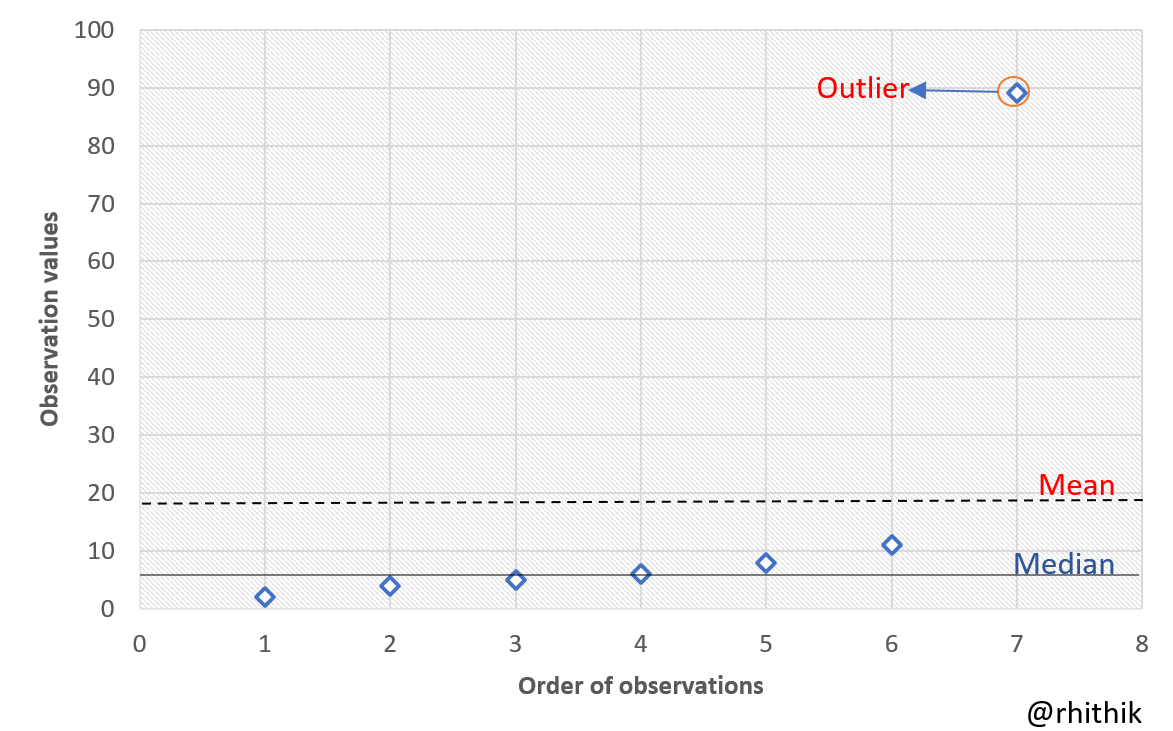
By just looking at the data, it can be said that the average would be somewhere around 7 but since an extreme value like '89' is present, hence the mean is heavily affected. The mean doesn't make sense while the median does as it isn't affected by extreme values, and it passes through nearly all the data points.
However, there seems to be a hidden message within this… Are you aware of what it could be? Exactly! Median divides the data into two equal parts. But what if I want to divide the data into more equal parts?
Partition Values
These are the values that divide the data or series into a number of equal parts. They are graphically located with the help of a curve called the ‘cumulative frequency curve’ or ‘Ogive’. There are various types of partition values like —
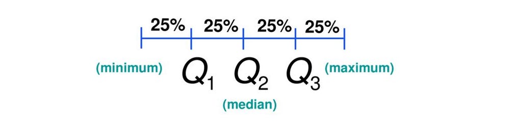
Quartiles - The 3 points which divide the data into 4 equal parts are called quartiles. For example, the first quartile ‘Q1’ contains 25% of the observations and is exceeded by 75% of the observations.

Quartiles Deciles - The 9 points which divide the data into 10 equal parts are called deciles. For example, the 6th decile ‘D6’ contains 60% of the data.
Percentiles - The 99 points which divide the data into 100 equal parts are called percentiles. For example, the 54th percentile ‘P54’ contains 54% of the data.
Anyway, the method for computing partition values is the same as those used for locating the median.

Mode
It is defined as the value that appears most frequently in a dataset. There can be more than one mode if multiple values are equally frequent (they are called ‘bimodal’ if there are 2 modes, ‘trimodal’ if there are 3 modes and so on). It is essentially the predominant value in the series.
When to use mode?
Categorical Data: The mode is particularly useful for categorical data where you want to know which is the most common category.
Multimodal Distributions: When the data has multiple peaks or clusters, the mode(s) can help identify these.
Describing Popular Choices: Useful in situations where the most common item, choice, or category is of interest.
Empirical Relationship
Usually when the data is symmetrical, the measures of central tendency tend to coincide each other at the center of the distribution. But when the data is skewed, Prof. Karl Pearson came up with the empirical relationship between the mean, median and mode as shown below -
Mode = 3*(Median) - 2*(Mode)

or

Mean - Median = 1/3rd of (Mean - Mode)
Which one is the best measure?
It is important to note that no measure is suitable for all practical purposes. But for different scenarios, there exists different measures. For instance, when the data is skewed, median is the best measure. When the data is original, both median and mean can be used. But when your data is categorical, mode is the best choice of measure.
Different mathematical formulas exist for different measures, which are to be used for the appropriate type of data — be it individual data, discrete data and continuous data. I’d suggest you check out YouTube for that, in case you decide to feed your curiosity!
Despite knowing these measures, there still lies a huge issue. This issue is indeed named, take note. However, before naming it, I believe it would be best to question the existence of this issue. What if I mention the average and expect you to come up with the whole data? Is it possible? If so, what are the measures required to come up with the distribution of values around the average? How do you find the ‘scatteredness’ of your data?
Alas, dear reader, you must linger a while longer to uncover the answers to these questions, but until that time,
'‘Once you stop learning, you start dying.'‘ - Albert Einstein
SUBSCRIBE TO THE STATISTICIAN
Outliers are data points that differ significantly from other observations in a dataset. They can be unusually high or low compared to the rest of the data and can distort statistical analyses, leading to misleading results. Median is a much suitable measure when the data contains outliers as mean is easily influenced by such extreme values.
A symmetrical distribution is a type of probability distribution where the left and right sides of the distribution are mirror images of each other. This means that the data values are evenly distributed around the central point, and the shape of the distribution is identical on both sides of the center.

A skewed distribution or an asymmetrical distribution is a type of probability distribution where the data values are not symmetrically distributed around the mean. In a skewed distribution, one tail is longer or fatter than the other. Skewness refers to the direction and degree of this asymmetry. They can either positively skewed (Mode < Median < Mean) or negatively skewed (Mean < Median < Mode).
